1. Simulation & testing ideas
2. Statistical analysis
3. Data mining and machine learning
4. Text mining and media analysis
Statistics with R
台南酷學園R語言推廣講座, April 2014
Johnson Hsieh (謝宗震)
Postdoctoral Reseracher in Biostatistics at NTHU
When to use R?
Simulation & testing idea in R
Monty Hall problem
假設你參加一個遊戲節目,你被要求在三扇門中選擇一扇:其中一扇後面有一輛車;其餘兩扇後面則是山羊。你選擇一道門,假設是一號門,然後知道門後面有甚麼的主持人,開啟了另一扇後面有山羊的門,假設是三號門。他然後問你:「你想選擇二號門嗎?」轉換你的選擇對你來說是一種優勢嗎?


http://en.wikipedia.org/wiki/File:Monty-CurlyPicksCar.svg
http://en.wikipedia.org/wiki/File:Monty_open_door.svg
Monty Hall problem
假設你參加一個遊戲節目,你被要求在三扇門中選擇一扇:其中一扇後面有一輛車;其餘兩扇後面則是山羊。你選擇一道門,假設是一號門,然後知道門後面有甚麼的主持人,開啟了另一扇後面有山羊的門,假設是三號門。他然後問你:「你想選擇二號門嗎?」轉換你的選擇對你來說是一種優勢嗎?
B <- 10000
x <- y1 <- y2 <- rep(0,B)
for(i in 1:B){
  x[i] <- sample(1:3,1)
  y1[i] <- 1
  y2[i] <- ifelse(x[i]==1, sample(c(2,3),1), x[i])
}
data.frame("keep"=mean(x==y1), "change"=mean(x==y2))
   keep change
1 0.337  0.663
Secretary problem
要聘請一名秘書,有 \(n\) 個應聘者。每面試一人後就要決定是否聘他,如果不聘他,他便不會回來。面試後總能清楚了解應聘者的合度,並能和之前的人做比較。問什麼樣的策略,才使最佳人選被選中的機率最大。
這個問題的最優解是一個停止規則。在這個規則里,面試官會拒絕頭 \(r - 1\) 個應聘者(令他們中的最佳人選為 應聘者 $M$),然後選出第一個比 \(M\) 好的應聘者。

http://www.wallpapergate.com/wallpaper22876.html
Secretary problem
n <- 8; reps <- 10^4; rec <- rep(NA, reps)
out <- data.frame("size"=n, "cutoff"=1, "successrate"=1/n)
for(r in 2:n){
  for(k in 1:reps){
   a <- sample(1:n) # rank of applicants
    comp <- min(a[1:r-1]) #best one befor rth applicant
    sec <- a[n] #Last one
    for(i in r:n-1){
      if(a[i] < comp){ #choose ith applicant better than comp
        sec <- a[i]
        break
      }
    }
    rec[k] <- sec
  }
  out[r,] <- rbind("size"=n, "cutoff"=r, "successrate"=sum(rec==1)/reps)
}
Secretary problem
out
  size cutoff successrate
1    8      1       0.125
2    8      2       0.326
3    8      3       0.401
4    8      4       0.411
5    8      5       0.382
6    8      6       0.322
7    8      7       0.232
8    8      8       0.121
out[which.max(out$successrate),]
  size cutoff successrate
4    8      4       0.411
Statistical analysis in R

http://arthritisbroadcastnetwork.org/2012/04/men-with-chronic-low-back-pain-may-have-reduced-bmd/
Bone Mineral Density
美國青少年脊柱骨質密度相對成長資料
資料來源:Bachrach et al. (1999)
library(ElemStatLearn)
data(bone) # BMD of 261 north american adolescents
bone[sample(nrow(bone), 8),]
    idnum  age gender   spnbmd
52     27 13.3   male  0.14382
479   377  9.6   male  0.01698
295   171 20.9   male -0.00498
333   208 13.1   male -0.02691
431   309 13.0 female  0.11171
87     47 12.7 female  0.05717
104    54 14.9   male  0.10294
270   149 12.8 female  0.08054
Bone Mineral Density
美國青少年脊柱骨質密度相對成長資料
觀察年齡與骨質密度相對成長之散佈圖

Bone Mineral Density
美國青少年脊柱骨質密度相對成長資料
觀察年齡與骨質密度相對成長之散佈圖

Bone Mineral Density
美國青少年脊柱骨質密度相對成長資料
以性別分組,觀察年齡與骨質密度相對成長之散佈圖

Bone Mineral Density
美國青少年脊柱骨質密度相對成長資料
利用平滑曲線法 (smooth splines) 觀察不同性別之趨勢

Bone Mineral Density
# 骨質密度成長率 vs 年齡
plot(spnbmd ~ age, data=bone, xlab="Age", ylab="Relative Change in BMD")
abline(lm(spnbmd ~ age, data=bone), lwd=2)

# 以性別分層
plot(spnbmd ~ age, data=bone, col = ifelse(gender=="male", 4, 2),
     xlab="Age", ylab="Relative Change in BMD")
legend("topright", c("male", "Female"), col=c(4, 2), pch=1, bty="n", cex=1.2)

# 平滑曲線分析
sp.male <- with(subset(bone,gender=="male"), smooth.spline(age, spnbmd, df=12))
sp.female <- with(subset(bone, gender=="female"), smooth.spline(age, spnbmd, df=12))
plot(spnbmd ~ age, data=bone, col = ifelse(gender=="male", 4, 2),
     xlab="Age", ylab="Relative Change in BMD", pch=1)
lines(sp.male, col=4, lwd=5)
lines(sp.female, col=2, lwd=5)
legend("topright", legend=c("male", "Female"), col=c(4, 2), lwd=2, bty="n", cex=1.2)
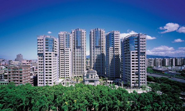

帝寶房價預測
- 資料來源:不動產實價登錄資料 (2012年8月 ~ 2013年9月)
- 頂級豪宅 40 / 21530 件
- 加入物件的面積大小、是否購買車位、屋齡、行政區域、樓層高低等因子配適模型
library(mgcv) #provides functions for generalized additive modelling
dat1 <- readRDS("dat1.rds")
# fit linear model
g1 <- lm(log10(總價)~面積+車位+屋齡+行政區+floor, data=dat1)
# fit addiive model with two smooth terms
g2 <- gam(log10(總價)~s(面積)+車位+s(屋齡)+行政區+floor, data=dat1)
# Compare adjusted R-squared, 越趨近1模型配適度越好
data.frame("linear model"=summary(g1)$adj.r.sq, "additive model"=summary(g2)$r.sq)
  linear.model additive.model
1        0.732          0.935
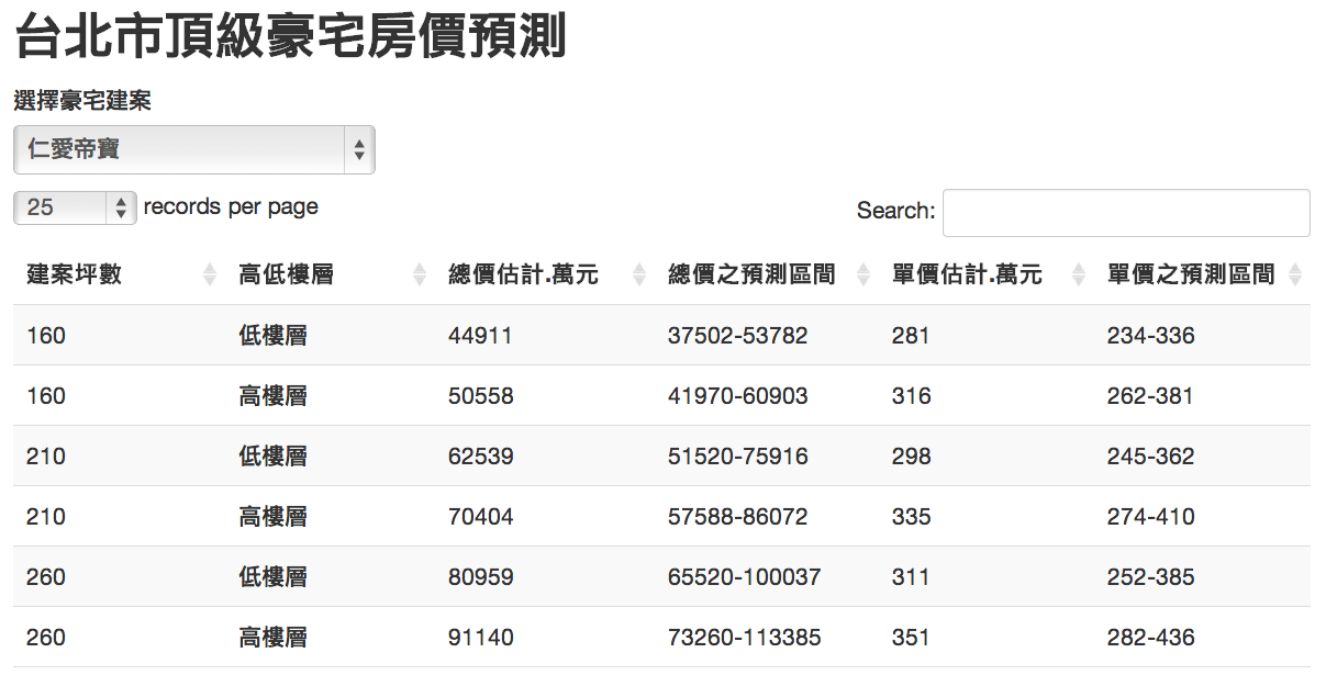
帝寶房價預測

帝寶房價預測
# set dataset, 帝寶格局
new <- dat1[1:6, c(2,3,4,6,7,12)]
rownames(new) <- 1:6
new$面積 <- c(160,160,210,210,260,260)
new$車位 <- rep("有車位",6);
new$屋齡 <- rep(8, 6)
new$行政區 <- rep("大安區",6)
new$floor <- rep(c("低樓層","高樓層"),3)
# prediction
tmp <- predict(g2, newdata=new, se.fit=TRUE)
pred <- 10^cbind(tmp$fit, tmp$fit-tmp$se.fit, tmp$fit+tmp$se.fit)
data.frame("建案坪數"=new$面積, "高低樓層"=new$floor,
           "總價估計.萬元"=round(pred[,1]/10000),
           "單價估計.萬元"=round(pred[,1]/10000/new$面積))
帝寶房價預測 (http://goo.gl/vT1Smr)

 http://www.bio1000.com/news/1/1867.html

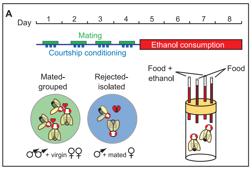
Shohat-Ophir, G., et al. (2012) https://www.sciencemag.org/content/335/6074/1351
Shohat-Ophir, G., et al. (2012) https://www.sciencemag.org/content/335/6074/1351
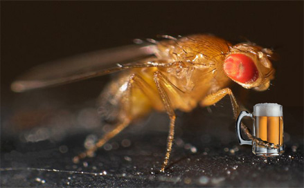
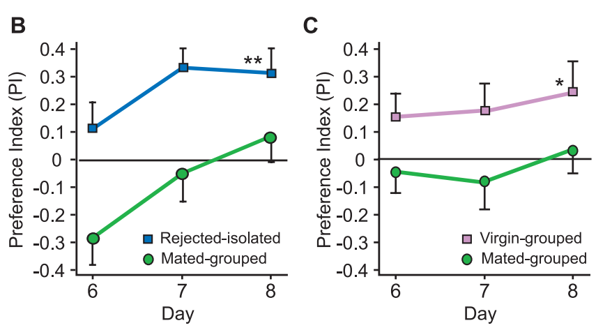
借酒澆愁愁更愁-探討果蠅求偶被拒絕與其飲酒行為之關聯性
- 學校名稱:國立科學工業園區實驗高級中學
- 作者:陳慶豐、陳昌逸; 指導老師:馮蕙卿、揭維邦
# raw data
dat <- data.frame(id=rep(1:8, each=2),
                  type=rep(c("glucose", "ethanol"), times=8, each=1),
                  group=rep(c("reject", "mate"), times=1, each=8),
                  ml=c(2.054, 3.677, 1.626, 3.078, 1.840, 3.378, 2.054, 2.694,
                       2.054, 2.993, 3.680, 2.223, 2.097, 2.608, 3.337, 1.753))
head(dat)
  id    type  group   ml
1  1 glucose reject 2.05
2  1 ethanol reject 3.68
3  2 glucose reject 1.63
4  2 ethanol reject 3.08
5  3 glucose reject 1.84
6  3 ethanol reject 3.38
借酒澆愁愁更愁-探討果蠅求偶被拒絕與其飲酒行為之關聯性

借酒澆愁愁更愁-探討果蠅求偶被拒絕與其飲酒行為之關聯性
tmp <- rep(0, 8)
for(i in 1:8) {
  tmp[i] <- ((dat$ml[2*i] - dat$ml[2*i-1])/(dat$ml[2*i] + dat$ml[2*i-1]))
}
out <- data.frame("reject"=tmp[1:4], "mate"=tmp[5:8])
PI.mean <- apply(out, 2, mean)
PI.sd <- apply(out, 2, sd)
library(Hmisc)
par(cex=1.2)
errbar(x=1:2, y=PI.mean, yplus=PI.mean+PI.sd, yminus=PI.mean-PI.sd, las=1,
       xaxt="n", xlim=c(0.5,2.5), xlab="", ylab="Preference index", cex=1.5, lwd=2)
axis(1, at=1:2, c("Reject", "Mate"))
abline(h=0, lty=2)
 http://i.gbc.tw/gb_img/5/001/991/1991405.jpg
LoL口袋深度分析
口袋深度:玩家在達到多少勝場時,能夠運用的英雄數量
英雄聯盟中可供使用的英雄有100種以上,英雄與英雄之間有若干相剋情形
會使用的英雄越多被針對的程度越低,因此口袋深度是判斷一個玩家程度的重要指標
library(devtools)
install_github('iNEXT','JohnsonHsieh') # http://johnsonhsieh.github.io/iNEXT/
library(iNEXT) # Chao et al. (2014)
source_url("https://gist.github.com/JohnsonHsieh/8389618/raw/qurey.R") # 戰績網查詢
id1 <- clean_lol("Toyz"); id2 <- clean_lol("AZB_TPA_Morning")
out <- list("Toyz"=id1$win, "Morning"=id2$win)
names(out[[1]]) <- id1$name; names(out[[2]]) <- id2$name
lapply(out, function(x) x[x>0])
$Toyz
奧莉安娜   奈德麗       慎   布里茨   歐拉夫     飛斯     露璐   希維爾   希格斯 艾妮維亞     李星
       7        7        2        7        3        3        3        4        2        1        3
  瑟雷西 古拉格斯     凱爾     犽宿 伊澤瑞爾   索拉卡
       4        1        1        1        2        1
LoL口袋深度分析
LoL口袋深度分析 (http://goo.gl/KngyYO)
out1 <- iNEXT(id1$win, endpoint=100); out2 <- iNEXT(id2$win, endpoint=100)
par(family="STHeiti")
plot(out1, ylim=c(0,40), main="口袋深度分析", xlab="勝場數", ylab="英雄個數")
lines(out2, col=2)
legend("topleft", c("Toyz", "AZB_TPA_Morning"), col=1:2, pch=19, bty="n", lty=1)

Data mining and machine learning in R

http://www.motherjones.com/files/images/Blog_Obama_Clinton.jpg
The Obama-Clinton Divide
primary = read.csv(url("http://www.stat.ucla.edu/~cocteau/primaries.csv"), head=TRUE)
primary$black06pct <- primary$black06/primary$pop06
primary <- subset(primary, state_postal!="MI")
primary <- subset(primary, state_postal!="FL")
primary <- subset(primary, !(state_postal=="WA" & racetype=="Primary"))
primary.sub <- subset(primary, select=c(county_name, region, winner,
                                        clinton, obama, pct_hs_grad, black06pct))
head(primary.sub)
  county_name region  winner clinton obama pct_hs_grad black06pct
1     Autauga      S   obama    1760  2268       0.787     0.1721
2     Baldwin      S clinton    6259  5450       0.820     0.0964
3     Barbour      S   obama    1322  2393       0.646     0.4627
4        Bibb      S clinton     922   755       0.632     0.2190
5      Blount      S clinton    2735   617       0.705     0.0155
6     Bullock      S   obama     471  2032       0.605     0.6982

The Obama-Clinton Divide
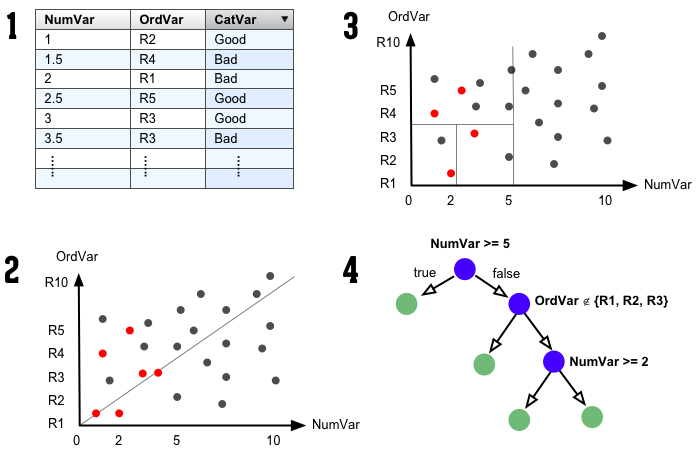
library(rpart) # Recursive partitioning
library(rpart.plot) # Fancy tree plot
library(RColorBrewer) # Nice color palettes
fit = rpart(winner~region+pct_hs_grad+black06pct,data=primary)
c1 <- ifelse(fit$frame$yval==1, brewer.pal(9, "Greens")[9], brewer.pal(9, "Blues")[9])
c2 <- ifelse(fit$frame$yval==1, brewer.pal(9, "Greens")[2], brewer.pal(9, "Blues")[2])
prp(fit, type=2, extra=1, col=c1, box.col=c2, shadow.col="gray")
The Obama-Clinton Divide

How do decision tree work

Handwritten digits
library(ElemStatLearn)
data(zip.train)
dat <- zip.train[which(zip.train[,1]==3),]
tmp1 <- tmp2 <- list()
for(i in 1:9){
  for(j in 1:7){
    tmp1[[j]] <- zip2image(dat, i+(j-1)*5)
  }
  tmp2[[i]] <- do.call("cbind", tmp1)
}
im <- do.call("rbind",tmp2)
image(im, col=gray(256:0/256), xlab="", ylab="", axes=FALSE)
Handwritten digits
以Principal Component Analysis (PCA) 進行手寫學習

pca <- prcomp((dat[,-1]))
b1 <- b2 <- round(seq(-4, 4, l=5),1)
par(mfrow=c(1,3))
image(matrix(pca$center,16,16),col=gray(256:0/256), main="Mean")
image(matrix(pca$rotation[,1],16,16),col=gray(256:0/256), main="PC1")
image(matrix(-pca$rotation[,2],16,16),col=gray(256:0/256), main="PC2")
Handwritten digits
以Principal Component Analysis (PCA) 進行手寫學習

Handwritten digits
tmp3 <- tmp4 <- list()
for(i in 1:5){
  for(j in 1:5){
    tmp3[[j]] <- matrix(pca$center,16,16) +
                 b1[i] * matrix(pca$rotation[,1],16,16) +
                 b2[j] * matrix(-pca$rotation[,2],16,16)
  }
  tmp4[[i]] <- do.call("cbind", tmp3)
}
pc.im <- do.call("rbind",tmp4)
plot(pca$x[,1:2], col=3, xlim=c(-6,6), pch=19, cex=0.5, panel.first = grid(6,6,1,2))
abline(v=0, col=gray(0.2), lwd=2)
abline(h=0, col=gray(0.2), lwd=3)
points(x = rep(b1,each=6), y=rep(b2, times=6), col=2, pch=19)
image(pc.im, col=gray(256:0/256), zlim=c(-0.8,1.2), axes=FALSE, xlab="PC1", ylab="PC2")
axis(1, at=seq(0,1,l=5), labels=b1)
axis(2, at=seq(0,1,l=5), labels=b2)
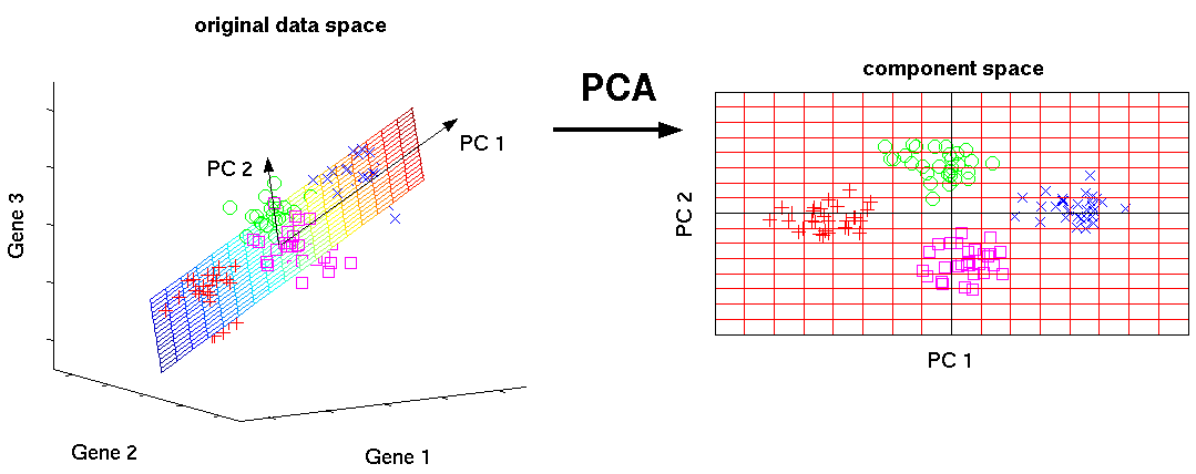
Basic idea behind PCA
 http://www.nlpca.org/fig_pca_principal_component_analysis.png
Text mining and media analysis in R
 http://juan.tw/?p=2269
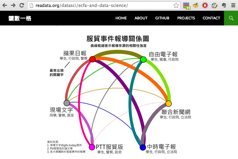 http://readata.org
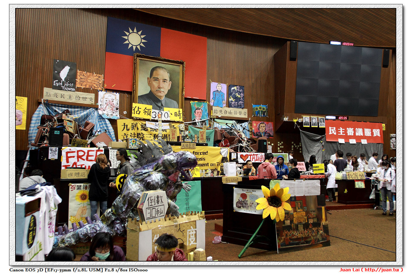
太陽花學運 文字轉播紀錄
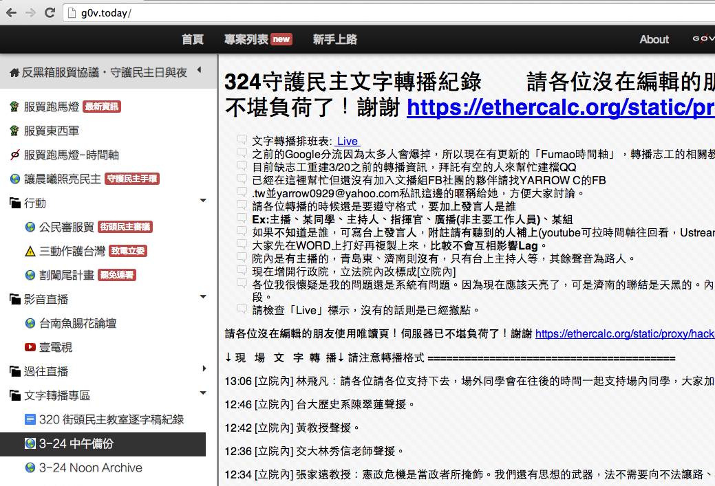
太陽花學運 文字轉播紀錄
verb <- iconv(readLines("news/live-text-0324.txt"), from="big5")
verb <- verb[-which(verb=="")]
verb[c(451, 400, 360, 200, 46, 12)]
[1] "魏楊:如果任何一個門被警察攻陷,不要往前推,慢慢往後退,退回廣場,坐下,幫我把這件事告訴每個門的指揮,如果任何門被攻破,慢慢後退,到廣場坐下!"
[2] "02:29 [行政院] 主持:各位朋友我們還是盡可能的守到早上,但是如果情況緊急的話,我們也不會強迫大家坐在這裡,大家還是保護自己的人身安全好不好"
[3] "03:14 [行院前] 糾察:等一下警察來抬你的時候,不要反抗,反抗的話他們也會很激動,他們都有帶警棍,請全身放軟讓他們不好抬。"
[4] "09:45 [立院內] 林飛帆:現在很清楚,有各式各樣意見,我們都尊重。但我們佔領國會是因為國會已經失靈,目的很清楚,就是要讓它發揮功能。我們在做的事情很簡單,我們沒有企圖代表所有不同的意見。無法發揮功能的國會,這才浪費人民公帑。我想我們清楚,昨天進到行政院的公民朋友,這裡面的組成有各式各樣的人。說不定有偷竊、偷吃蛋糕的行為,這些行為我們都不鼓勵,如果真的有這種事情發生,蕭家齊可以請警方蒐證。"
[5] "19:20[立院內]廣播:同學請看看前面這一袋物資(垃圾包成一袋),請不要這樣,我們沒有人有義務要幫你們收垃圾,跑社運的人愛回收好嗎!(歡呼)各位看看這個咬一口排骨就丟的便當,我以後不要再看到這個了好嗎?以後再讓我看到,我只叫麵包。"
[6] "23:20[青島]教授:我舉個服貿的例子:台灣不缺醫院,但是若是讓陸資介入,可能會改變目前台灣的醫療品質,我們的自費額可能增加,雖然是台灣員工醫台灣病人,但決策者是對岸的董事,那台灣在陸資為主的產業中沒有發言權。中立的民眾,現在是該表態的時刻了,表態後民主才能被尊重。(民眾:好!)"
太陽花學運 各家媒體報導內容
content <- read.csv("news/five-news-0324-utf8.csv")
names(content)
[1] "新聞來源" "發佈時間" "網址" "標題" "內容" "發佈日期"
content[c(9, 301, 880, 1255, 1732), c(1,2,4)]
     新聞來源        發佈時間                                 標題
9        台大 2014/3/24 21:15                                 <NA>
301      中時 2014/3/24 20:14            服貿衝突 國際媒體大幅報導
880      自由 2014/3/24 12:07  遍地開花》香港學聯 聲援台灣學生示威
1255     聯合 2014/3/24 14:58 強勢驅離共174人受傷,其中119名是員警
1732     蘋果 2014/3/24 20:24             蘋論:不容鎮暴警再打學生
媒體報導內容分析
# 計算各家媒體的關鍵字頻
source("src/tm.R")
myNews <- list()
myNews[[1]] <- myDocTerMat(docs=verb, method="vec", clean=FALSE)
for(i in 1:5){
  id <- which(content$新聞來源==levels(content$新聞來源)[i])
  input <- as.character(content[id,"內容"])
  myNews[[i+1]] <- myDocTerMat(docs=input, method="vec")
}
# 計算各家媒體的關鍵字頻(續)
dat <- lapply(myNews, function(x) x$fre)
u <- as.character(unique(unlist(lapply(dat, function(x) as.character(names(x))))))
tmp <- lapply(dat, function(x) rep(as.character(names(x)), x))
tab <- do.call("rbind", lapply(tmp, function(x) table(factor(x, levels=u, labels=u))))
rownames(tab) <- c("現場", levels(content$新聞來源))
tab <- tab[, order(colSums(tab), decreasing=TRUE)]
tab[,1:10]
     學生 行政院 服貿 民眾 警方 政府 反服貿 警察 立法院 魏揚
現場  113    201   68   54   10   65      7  180     57   68
聯合 1177    660  416  402  330  236    347  118    270  109
蘋果 1436    513  428  308  357  299    214  248    211  195
台大  163     60   83   57   23   43     27   52     31   39
中時  966    475  354  195  220  133    187  102    149  182
自由 1424    479  491  248  250  296    160  212    190  223
媒體報導關聯性

媒體報導關聯性
library(vegan)
library(igraph)
termMatrix <- 1 - as.matrix(vegdist(tab, method="horn"))
g <- graph.adjacency(termMatrix, weighted=T, mode = "undirected")
g <- simplify(g)
set.seed(1016)
layout1 <- layout.fruchterman.reingold(g)
w <- 10^(E(g)$weight)
E(g)$width <- 15*((w-min(w))/(max(w)-min(w))) + 0.2
E(g)$color <-  sample(colors()[30:300], length(E(g)$weight))
node_size <- unlist(lapply(myNews, function(x) ncol(x$tdm)))
V(g)$size <- scale(node_size, center=FALSE)*70
V(g)$label <- V(g)$name
plot.igraph(g, layout=layout1, vertex.label.family="STHeiti", vertex.label.cex=1.4)
Resources
| Useful R websites | Basic statistics book with R | Advanced statistics book with R |

|

|
Come back for more
- Sign up at: www.meetup.com/Taiwan-R/
- Give feedback at: www.facebook.com/Tw.R.User
- MLDM Monday VOD at: www.youtube.com/user/TWuseRGroup